How MoonDream Works

I discovered MoonDream watching an AI engineer talk of how small model slaps. I have seen enough talks on people trying to sell finetuning small models but I haven't been particularly impressed by most of their performance out of the box. It felt like many people skipped the data preparation part of finetuning and opting instead for the more intellectually stimulating algorithms and model optimisations. While useful, I do not believe they satisfy the Pareto principle for Ai model building.

Running it locally, I had fairly impressive results - not surprising given he even gave a live demo of the model at some point. You typically don't do this without a significant amount of confidence in the model's performance.

So, how did he enable a large language model to "see"?

I've seen a lot of machine learning engineers try this. It's a really hard problem and this remains the first attempt I've seen successful on small LLMs.

So what did he do differently?

Below, I share some notes I took while reading through the code of the architecture.

Data Preparation

When preparing synthetic data, the MoonDream team found that the models hallucinate heavily with VLM understanding

Sophisticated Synthetic Data Processing Pipeline

Processing pipeline included:

Correct transcription errors
Extract list of facts
Validate each fact against the original transcription
Convert facts to question/answer pairs
Filter out unhelpful pairs (e.g. how many people are in the image? There are people in the image)
Generate "absurd" / irrelevant questions to serve as distractions

Synthetic questions are, however, usually not representative of real-world user queries.

Therefore, when you ask a model to generate "user queries", it will aim to preserve diversity from the original dataset to avoid "model collapse" - when the model just defaults to something weird or stupid.

Architecture

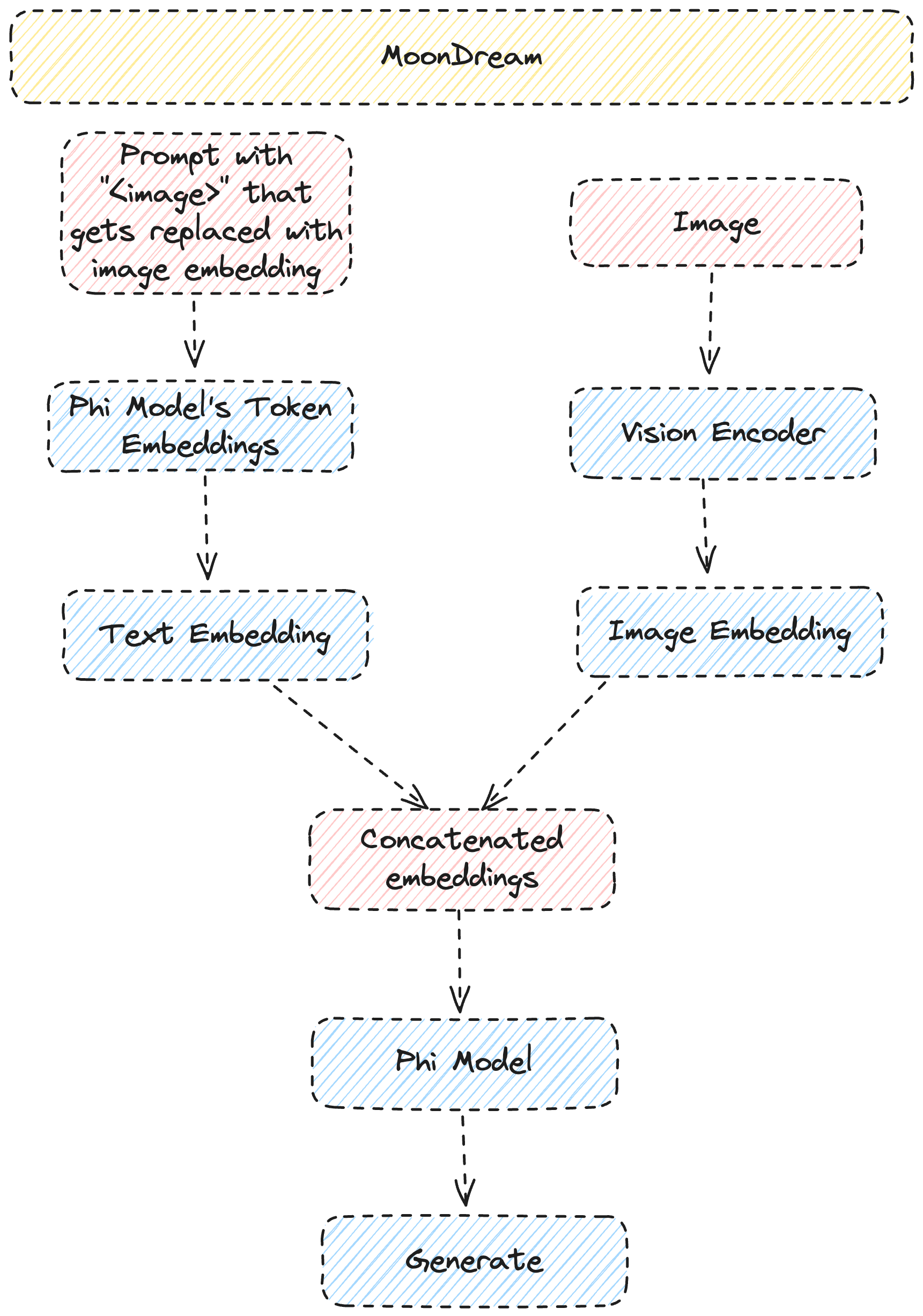
MoonDream's architecture is extremely interesting. Let's dive in. We share a high-level overview of MoonDream's (relatively simple) architecture below.

MoonDream Architecture

Vision Transformer

Transform the input image into patches and linearly projects them into embed_dim dimensions. This is the first step in making an image suitable for transformer processing.

Positional embeddings allow transformers to learn spatial relationships. Could use RoPE embeddings instead?

Instead of using CNNs that process local regions with convolutions, transformers can attend to the entire image through self-attention.

Patch-based approach and not pixel-level approach. Instead of pixel-level processing, the image is divided into patches and treated as a sequence.

Explicit positional embeddings provide spatial information normally implicit in CNNs.

Fourier Features

Fourier feature maps input data into higher-dimensional feature space. This creates a richer gradient space to improve back propagation efficiency.

Vision Encoder

def vision_encoder(input_BCHW: torch.Tensor, w: VisionModel):
    x = rearrange(
        input_BCHW,
        "b c (h p1) (w p2) -> b (h w) (c p1 p2)",
        p1=w.patch_size,
        p2=w.patch_size,
    )  # B3HW -> B(HxW)(3xP1xP2), aka BTC

    x = linear(x, w.patch_emb)
    x = x + w.pos_emb
    for block in w.blocks:
        x = x + attn(layer_norm(x, block.ln1), block.attn)
        x = x + mlp(layer_norm(x, block.ln2), block.mlp)
    x = layer_norm(x, w.post_ln)

    return x

The rearrange method transforms image data into something useful for a vision transformer. This divides the input image into fixed-size patches. The input tensor has shape (batch, channels, height, width) and is reorganized into a sequence of flattened patches.

Some unique properties of the vision encoder - it reads in a vision layer, and then it reads in a unique model type.

Weight Tying

Weight tying is where the input embedding and output embedding layer shares the same weights. Interesting results.

There are 2 main reasons to perform weight tying according to this Reddit thread.

Reduces memory footprint by eliminating 1 of 2 large parameter matrices in LLMs
Results in better and faster outcomes (although I am skeptical)

In most situations, the output generation probability distribution is going to be significantly different from the incoming generation probability distribution.

However - it required assuming the distributional hypothesis.

How Moondream works